In LTspice, mathematical expressions are best suited for behavioural sources, which are extremely versatile, but they come at a price: simulation slowdowns as the processed numbers go higher. The simplest, most relevant example possible is a simple repeater:

V1 in 0 SIN(0 1k 1)
B1 out 0 V=V(IN)
.tran 10

This will not run as fast as:

V1 in 0 SIN(0 1k 1)
E1 out 0 in 0 1
.tran 10

Note that if the old notation is used:

E1 out 0 VALUE={V(in)}

LTspice will replace the VCVS with a B-source, internally, something easily verfied by checking generate expanded listing in the control panel, which will result in the error log showing:

b§e1 out 0 v=v(in)

(only true for old-style expressions such as POLY, or even LAPLACE, on two-pin E or G-sources).

B-sources have two parameters, tripdv and tripdt, to help with these cases. As the frequency is increased and the simulation time adjusted to run the same number of periods (10), it will start to go faster and faster. This means that there are some default settings for tripdv, tripdt.

But this is just a repeater, if functions come into play, for example:

V1 a 0 SIN(0 1k 2)
V2 b 0 SIN(0 2k 1)
B1 out 0 V=V(a)*V(b)
.tran 10

Things get a bit different. Still, as above, it will run faster with increasing frequency, and for various settings of tripdv, tripdt but, in order for these two to be useful, the simulation needs to be started, evaluate the run, then stop it, tweak the two parameters, then re-run the simulation. Multiplication is not the only one affected.

This prompted me to look for alternatives. First, E and G-sources are the fastest primitives (and their F and H cousins), but they only perform linear multiplication. Since even the manual (bottom note)↗ mentions about favouring VCCS over VCVS, one of the most obvious solutions was replacing one of the behavioural variables, and then use Ohm's law: V=R*I, with I provided by a G-source and R by a behavioural resistor:

V1 a 0 SIN(0 1k 2)
V2 b 0 SIN(0 2k 1)
G1 0 out a 0 1
R1 out 0 R=V(b)

This does increase the speed of the simulation, but the zero crossings can prove problematic, even more so in feedback loops. Besides, it's still using a behavioural expression, so to replace it, the only two other options for a variable resistor, as simple as possible (MOS is too complex), would be the A-device VARISTOR (but that has a fixed, linear variable resistance), or the VCSW with negative hysteresis. The CCSW needs a current sensor, that means one possible extra element/node.

Now the problem is creating a control voltage, that is nonlinear in its nature, and which needs to vary the resistance of the VCSW according to V(b). Placing a 1A current source across the VCSW will give a voltage proportional to its resistance, so if that is incorporated within a loop, the control voltage can be obtained. One more thing to take care of is the negative input swings:

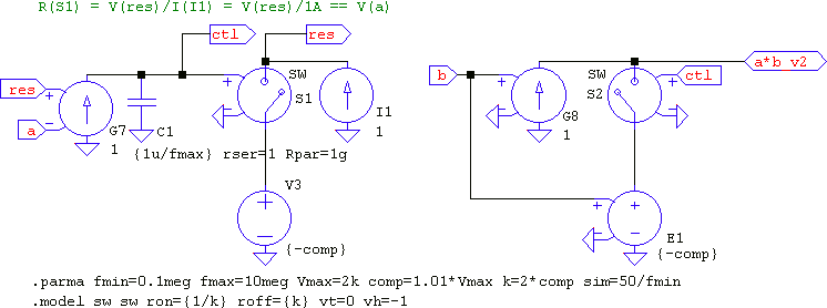
I1 across S1 generates V(res), which is compared to V(a), then run through the loop filter made of G7, C1, which create V(ctl); V3 allows negative values, same as E1. Any VCSW controlled by V(ctl) will have its resistance vary according to V(a). To test, G8 has V(b) as input, and S2 as the variable resistor. This will give the resultant A*B and fly in any condition, despite having so many elements.

But it's far from perfect: for one, the resistance of the switch must accomodate the voltage swing of V(b), that is, Ron=1/max(V(a)), Roff=max(V(a)), their values covered by k, which is (generously) chosen as twice the value of comp, which covers the input swing, which is set by Vmax, representing an estimate of the maximum input values. Then the loop filter, a simple PI, must have enough gain for the whole bandwidth, estimated with the value of C1, to have at least 6 decades. So, it's fast, but too much hassle.

Another alternative is using the Vto and dir in the VCCS value field↗. This allows for a quadratic expression that will run extremely fast in any conditions, but, because of Vto, creating a true A² for a bipolar input requires one of two methods:

1. Estimate the input swing and set Vto<-max(V(in)), which makes the output appear as (A - ε)² = A² - 2Aε + ε², thus the need to subtract the two unneeded terms in order to remain with the desired A², and provide the estimate, or
2. Use two quadratic VCCSs, with Vto=0 and different signs.

The first choice is not very appealing because there is a need of an estimate and use its squared value for subtraction (right, I1), and the second has two quadratic sources for one quadratic output (left):

Since a G-source has a positive and a negative input, (A - B)² can be achieved, but which creates two additional, unneeded terms; these can be subtracted: (A - B)² = A² - 2AB + B² ⇒ 2AB = A² + B² - (A - B)².

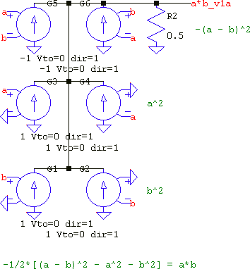
But now there are six quadratic sources performing one multiplication. This can be reduced by considering that: (A + B)² - (A - B)² = 4AB, which means that for the price of a sign inversion for V(b), two quadratics can be eliminated:

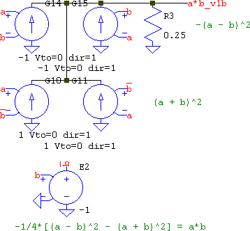
Still, while the operation is very fast and accurate, there are four quadratic operations for a multiplication. Fortunately, LTspice provides an A-device that is tersely listed in the official help file, but it is explained in more detail in the undocumented ltwiki↗; one of the most versatile elements. LTspice XVII↗ now has a dedicated symbol for it, but in LTspice IV↗ there wasn't any. Here, I'll be using LTspice XVII's symbol, but if LTspice IV is the tool of choice, unless there is a custom symbol, IMHO the best, ready-made symbols to use with it are the AND, OR, or XOR gates, since they provide 5 input pins (out of which only 4 are needed) plus complementary outputs (out of which only the direct output will be used, practically); but, of course, it's a choice, not the law. The multiplication now is as easy as this, and it's as fast and accurate as it gets:

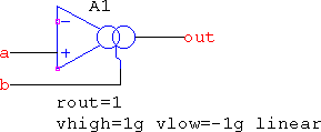
Note that the linear mode is used, to avoid unneeded distortions. It's still not perfect since it relies on setting the upper and lower limits, more on this later below.

So, multiplication is taken care of, what about division? There is no element that does it natively, so maybe look at the problem from a different angle. Enter implicit math: A/B=Y ⇒ A=YB. A and B are known, multiplication can be done, all that's left is to find a way so that Y can be found out. The method used earlier, VCCS+VCSW as a multiplier, can be emulated in a different way:

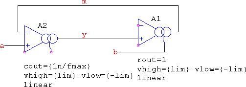
A2 uses only its first two inputs, thus it's a basic differential amplifier, with y=a-m as its output. A1 uses both differential inputs, and has m=y*b as its output. This means a=m=y*b which is an implicit way of saying y=a/b. We simply let LTspice calculate it automatically based on the would-be loop filter made of A2 as an integrator. This is not perfect, either, since, like in the VCCS+VCSW case, the estimation of the bandwidth of the input signals is still present in the loop filter, and the differences compared to a true division are dependent on it, but they are not large. For example, if V(a) is a sine of ±1kV peak and V(b) is a sine in the range of 1mV..3mV, with a frequency sweep from 1MHz..10MHz (it's all in the downloads), the difference looks like this:

It might look huge, until you consider the output, at which point float comes to mind:

Not only the simulation is unstoppable, but the differences get smaller as the timestep is smaller, and can get even smaller if higher bandwidth is used. Or simply use a huge, flat gain, if you feel lucky. It will work for "static" experiments, but when dynamics come into play, an integrator is needed, even a zero sometimes, so A1 may need replacing with a VCCS+C:

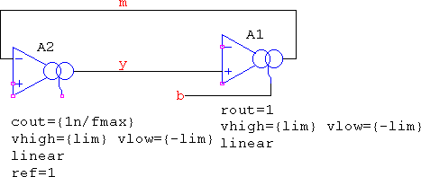
So, if division is possible, inversion is even easier, by setting the internal parameter ref=1 in A2, and giving up the a input, which results in 1=m=y*b ⇒ y=1/b:

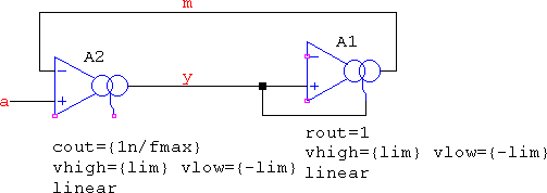
What about square root? In this case, keep the a input, and transform the b input into y, so that the output is a=m=y*y, or a=y:

However, sqrt() comes at some prices for negative inputs. Since LTspice doesn't calculate using complex numbers in .TRAN, the square root of negative values come out as zero. The implicit square root, though, has problems getting over them, and for good reason, so some trickery is needed. First, the input needs to be converted using the equivalent of the uramp() function (discard negative values). This can be achieved with a computationally cheap table(0,0,{lim},{lim}), but testing revealed that this is not enough, since the output tends to go negative, despite the explicit setting of vlow=0.

The explanation is that, similar to the SAMPLEHOLD, for linear mode, the OTA doesn't actually limit the output, i.e. vhigh and vlow are not the absolute limits. Instead, it has a parameter rclamp, which is swapped with rout when the limits are reached. With the default values, for the OTA, rclamp=1, thus the amplification is halvened, and for the SAMPLE, rclamp=1m), thus the amplification is reduced by a factor of (almost) 1000x. This means that due to the loop filter's settling times and despite the explicit setting of vlow=0, the output can get negative, so the equivalent of the abs() function is needed.
 A cheap table({-lim},{lim},0,0,{lim},{lim}) can be used. Using table() means the OTA uses linear mode. To help deal with the discontinuities, a small value for cout is a good idea. An alternative is using the parameter epsilon, which works just like in the ideal diode, but since this will be added to the output OTA, it can distort the output. The capacitor also adds distortion, but it's directly related to bandwidth, rather than voltage level, so it's preferred. Unfortunately, testing also showed that discarding the input uramp() in the favour of this last abs() is not possible, but the abs() can be omitted if A1 is used with soft limiting (isrc and isink set), but only with the asym flag, otherwise the midpoint is shifted to be (isrc-isink)/2. The final result is this:

a⁺=uramp(a), |y|=abs(y), in rest, nothing changed.

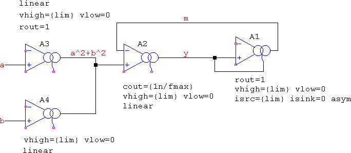
With these, hypot(a,b) almost invites itself now: first, a and b need to be squared and summed, which means there will be no negative values, so the uramp() input is no longer needed for the sqrt(). In rest, a² + b²=m=y*y=|y*y| ⇒a²+b²=y:

All the circuits presented above will outperform their behavioural expressions in speed, but may suffer from apparent minor inaccuracies. For the sake of a bit of innocent fun, logarithms and hyperbolic functions could be coerced into being. For the logarithm, ln(x)=∫1/x dx, from which division is possible and the integral part is a simple integration. Unfortunately, there is a vicious circle:

• Integration is a function of a time window, which means "static" values, such as ln(1.618) will not be possible, only for a range of time, which in turn means the need to apply that window to the integrator's gain, and
• The same integration, in order to output a true result, needs initial conditions, thus "static" logarithms, else the values will be shifted.

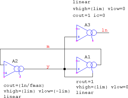
The result is what's seen below, with V1 providing a time-variable input (here, a basic ramp), A1, A2 performing implicit 1/x, and A3 performing the integration, with zero initial conditions:

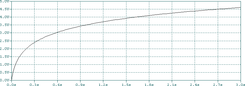
Even so, despite the difference between the lowest and highest values being true to a ln(x), x∈[0.3..30] plot, the Y axis is shifted because of the improper initial conditions:

Still, this proves that other, more exotic functions can be made, for example exp(x) and exp(-x), since one is the inverse of the other. In this case, though, the input must be of the form of a premade exponential, after which a simple 1/x will do. The signal could come from an RC lowpass driven with a step function, or LTspice's own EXP source. And, since these can be made, cosh(), sinh() and tanh() follow, while having the value of a kids' show: amusing, but forgettable.

If it's about tanh(), only, there's a simpler method. The soft-limiting of the OTA uses a tanh(). Forcing the limits to be ±1 means any ramp at the input will act as the X-axis for the tanh(). So use the OTA with vhigh=1 vlow=-1 rout=1 iout=1, and let a ramp be the driver. Or, you could make it asymmetric, vhigh=1 vlow=0 rout=1 isrc=1 isink=0, and make the ramp with half its end values; then the differentiator can have unity gain.

As a side note, an alternative to δ(t) is also possible. To avoid setting a very narrow pulse with sharp edges and very high values for testing the impulse response of filters, the equivalent formula↗ for the Dirac function is better suited for convergence. However, using it requires a behavioural source which would be limited for very low values of a. For example and by itself, only, with a=10u and 2s simulation time it will not show any response, so tinkering with tripdv and tripdt is needed, whereas using this setup, it will show the response, and it would not require timestep control:

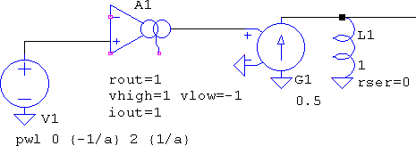
The trick is to use the derivative: d/dx tanh(x)=1/cosh²(x). The function has so many smooth derivatives it's completely oblivious to discontinuities, but the integral from (-∞,∞) is 2, while for δ it is 1, so the gain of the differentiator is 0.5 to account for the difference in the areas of the two functions. So, it's not quite Dirac, but close enough and, most importantly, smooth as factorial. As it is shown, the ramp makes the pulse be delayed for half the simulation time, so if more time is needed, simply extend the ramp. Since the ramp is provided by a simple PWL voltage source, its points will be known in both value and time prior to simulation start, so they will not cause problems.