Jump to downloads. This section will converge towards the reasons and methods I used when making the Filter, but these can be applied to any other usage of SPICE.

Since SPICE is meant to be an analog circuit simulator (even if some are mixed), when talking about filters two things come to mind: inductors and capacitors. These represent the states of the filter. And, unless the purpose of the simulation is to actually verify or test some filter configuration, using a filter in SPICE does not mean replicating the Sallen-Key circuit from the breadboard. Instead, what is of interest is its behaviour, since the simulation time is directly affected by the number of elements and nodes in the schematic. That is, all that's needed is the effect of the filtering, in the most efficient way possible.

---

Passive filters

Passive filters should not need any explanation, they're a simple case of "place and simulate".

---

Analog active filters

With these in mind, building a filter is easy. First, SPICE is a generic name for simulators, and each simulator will have its own tactics of solving the matrices. LTspice, in particular, uses the modified nodal analysis ↗, which means current sources are preferred to voltage sources. This is also mentioned in the help for the VCVS↗:

Note: It is better to use a G source shunted with a resistance to approximate an E source than to use an E source. A voltage controlled current source shunted with a resistance will compute faster and cause fewer convergence problems than a voltage controlled voltage source. Also, the resultant nonzero output impedance is more representative of a practical circuit.

Therefore all that's needed is to start with the basic formulas:

vC(t)=	1	∫0t	i(τ) dτ		vL(t)=	L	d	i(t)
	C						dt

which says that a current source plus a capacitor give a voltage that acts like an integrator, and with an inductor − a differentiator:

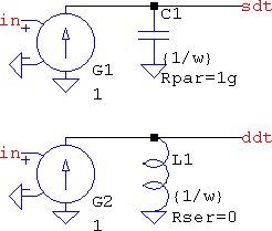
The file sdt,ddt.asc shows a comparison between these two and their behavioural countderparts. Using the primitives G+C and G+L will never need any tinkering with hidden parameters such as tripdv or tripdt for behavioural sources. Interfacing these with elements that consume current is not a good idea, though, unless some sort of buffering is used. All these are analog active filters, because their behaviour mimic active filters (the current source is an active element).

There are other ways. Among them LAPLACE and the FREQ sources, which are versatile, in particular the LAPLACE expressions, but they come at some prices. The FREQ source is the equivalent of the table() in time-domain: a piecewise linear function that tries to approximate a continuous frequency spectrum. Under the hood, it has the same approach like the LAPLACE source (quote from the help↗):

The time domain behavior is found from the impulse response found from the Fourier transform of the frequency domain response. LTspice must guess an appropriate frequency range and resolution. The response must drop at high frequencies or an error is reported.

In short, any frequency domain analysis (.AC, .NOISE, .TF) are absolutely fine, but any time domain can be a mess. It's not a guaranteed mess, but a possibility, whose chances of occurring increase with the complexity of the expressions. The FREQ source can benefit from more data points, which makes the resulting impulse response less noisy.

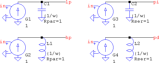
So, with integrators and differentiators any filter can be built. A 1st order lowpass can be built with a classic RC lowpass and a VCVS, which is fine, but that means having 3 elements and 2 nodes (3, with the input). Using a VCCS, a lowpass can be represented as an integrator with an extra parallel resistor, while a series resistor will change the transfer function into a PI filter:

HLP(s)=R∥	1	=	1/(RC)		HPI(s)=R+	1	= R	s+1/(RC)
	sC		s+1/(RC)			sC		s

Similarly, a differentiator with a parallel resistor will become a highpass, or a PD filter with a series resistance. The lowpass and the highpass can also be accomplished by using the integrator and the differentiator, respectively, and feeding their outputs back to their inverting inputs; they will be the same transfer functions, with the exception of having only one non-inverting input available. There is one small, hidden bonus: the capacitors can retain their 1/ω value while the VCCSs can have any value for the gain. This means that building the filter with a different corner frequency is as easy as defining a .param; there is no need to change the topology, only some value(s). See the file 1st_lp,hp,pi,pd.asc from the archive for examples.

Second orders are very posible. The undamped case is a simple series or parallel LC, it will be mentioned later. For the overdamped and critically damped situations, the denominator can be split into two real, 1st order equations. But the underdamped case can't be split since SPICE doesn't work with imaginary numbers in time domain. This means that, as far as the transfer function goes, there need to be two chained integrators. Since an RLC is a 2nd order circuit, it can be used to form a biquad. Kendall Castor-Perry's example↗ and accompanying symbol↗ (and not only↗) can be found in the LTspice group↗. But that's not the only way. Following the second canonical form, this is how the generic transfer function can be built:

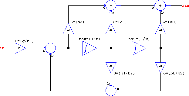
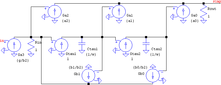
As nice as it may look, it's a waste in terms of computation. This is because every element is a subcircuit: the integrator is a VCCS and a capacitor (just like in the above), the gain is a VCCS plus a resistor, the difference is the same, and the summer has two VCCSs and a resistor. As far as the node count for each subcircuit, they're optimal (the sum of outputs + inputs), but the component count for the overall flattened netlist is: 6 x gains + 2 x integrators + 1 x difference + 3 x summers = 6*2 + 2*2 + 1*2 + 3*3 = 27 elements, while the node count is 13. They may all be linear, but that's still a lot for a simple 2nd order transfer function. If the subcircuits are replaced with their consituent primitives, the element count can be simplified: the summers and the gains can all be combined into a VCCS each, tied into a single node, and a single terminating resistance. Now the circuit has 8 x VCCS + 2 x resistors + 2 x capacitors = 12e, while the node count has dropped to 5! That's quite a dramatic reduction (see canonical.asc):

And yet, we can simplify it even more! The combined summers + gains can also be integrators. And if the circuit is rearranged to be in the first canonical form, the BOM amounts to 6 x VCCS + 2 x capacitor + 1 x resistor = 9e and 4n (Kendall's biquad has 5n; couldn't help it 😉). And the hidden benefit is the negative feedback for all the integrators, which improves stability.

This is as low as it can be ...or? There is a class of devices that are particular to LTspice, so using them will make the schematic incompatible with other simulators. They are the A devices↗. Among them is the OTA:

There is a special case of A-device called the OTA. It is a four-quadrant, multiplying, transconductance amplifier that is the corner stone of most of the Op-Amp macromodels in LTspice. The transfer function defaults to hyperbolic tangent. It supports input voltage and current noise densities that can specified as arbitrary equations of frequency and bias voltages. Both normal and common mode current densities are supported. If you use this device, please curve trace it's behavior to make sure you know what it is doing.

Unfortunately, the LTwiki help doesn't have this bit (yet), since it was only recently added into LTspice's help, so this is a quote straight from the official help (F1). It has many parameters, but among them is an output RC, which is builtin, like the parasitics for L and C. This means that they will not count towards the final node count since, as the good book says (from the capacitor↗, but valid for every element with parasitics):

It is computationally better to include the parasitic Rpar, Rser, RLshunt, Cpar and Lser in the capacitor than to explicitly draft them. LTspice uses proprietary circuit simulation technology to simulate this model of a physical capacitor without any internal nodes. This makes the simulation matrix smaller, faster to solve, and less likely to be singular at short time steps.

This means that the capacitors and the resistor can be eliminated, since they can be defined inside the OTA. The node count remains the same, but there are now only 6e; three less. Not bad, coming from the original 27e + 12n. However, using only G+C+R elements means this is compatible with a generic SPICE netlist. 2nd_generic.asc has this and the reduced version, as well as behavioural expressions based on the difference equation; they work better in .AC than they do in .TRAN, and the only reason they are shown is to know that it can be done that way, too, otherwise the G+C+R is preferred.

Now, this is a generic 2nd order transfer function, but the usual suspects are the particular cases like lowpass, bandstop, which means not all the elements will be needed. An all-pole lowpass has the transfer function:

H(s)=K⋅	a0
	s2+b1+b0

For a unity gain, a₀ = b₀, but have opposing signs (in the schematic), which means the feedback doesn't need to have two, distinct adders/subtractors; one VCCS is enough. It also doesn't have any a₁ or a₂ terms, which means any of the feed-forward VCCSs can be eliminated. Not only that, but a₂ is the only reason for which the b₂ VCCS was added, otherwise a strictly proper denominator is assumed. Therefore, all that's left are the two integrators. Alas, for pole-zero filters the only element missing will be a₁ (unless there is a special need for it). Again, the output is unbuffered, but if it's interfaced with pure voltage mode inputs, or very high impedances, this is no problem.

On the other hand, a highpass needs the feedforward path, which means keeping both the a₂ and b₂ terms, but only if the generic circuit is considered. What if this is thought of in terms of frequency transformations? A highpass is a lowpass with 1/s instead of s: H_HP(s) = H_LP(1/s). Instead of continuing with the transformation, mathematically, to end up at the s² numerator, why not consider that a capacitor, 1/(sC), represents the s term, which means 1/s = 1/[1/(sC)] = sC. So if the capacitor is replaced with an inductor of the same value in the circuit above, what results is a complementary all-pole highpass:

And here is one of the best parts. Applying frequency transformations for lowpass to bandpass means s → (s²+ω₀²)/(s⋅ω_bw), which is an ideal notch, the undamped case mentioned earlier, and which can be modelled by a simple parallel LC. The resulting order of the transfer function is doubled, but not the number of elements and nodes: the capacitors simply aquire a neighbour, an inductor, which means only two extra elements. And if LTspice is used then there will be no extra elements because the Cpar parasitic can be specified in an inductor. Their values will be the same 1/ω, but with an additional term representing the ratio between the central frequency and the bandwidth, the quality factor of the resulting bandpass. The previous circuits and the next one are from 2nd_lp,hp,bp,bs,ap.asc, where Q is the quality factor of the lowpass, wp is the pulsation of the center frequency (or the original lowpass), and Qr is the quality factor of the resulting bandpass:

Higher orders are, still, very possible. The same stability considerents apply here just like in any transfer function encompassing higher order polynomials. The filters can be broken down into 2nd order sections (± a 1st order one) and any high order filter can be simulated efficiently. But now another problem shows up: assigning the values for higher orders can be a problem if the filter needs to be changed. Possible scenario: due to some requirements, some 4th order Chebyshev is needed, but then the requirements change, or there is a need to adapt certain other aspects of the whole project, and the filter needs to be changed. Since this is not a simple matter such as changing a sign, or a value, most probably all the values will need changing (maybe except the capacitors, since they may only have 1/ω). And since a 4th order lowpass implies a minimum of two VCCSs and two capacitors, a minimum of 4 values need to be changed (possibly up to 8). Now, 4 values are nothing, by themselves, but there is also a matter of calculating the values, which means the task of dealing with the schematic is now hindered by the need to adjust the filter. For this, .param and .func to the rescue. canonical.asc already has something like this by using .param statements to automatically assign the biquad coefficients to the elements in the schematic, so the basis is already laid. All that's left is an automatic way of calculating them according to some rules.

In this case it's a Chebyshev filter↗ and calculating the coefficients for the biquad starts from the poles of the lowpass prototype. There is plenty of documentation about this, so I'll just ennumerate the formulas and the necessary steps. Since the filter will be split into 2nd order stages, the denominators will have real coefficients. Also because of the 2nd order splitting, there's no need to calculate all the complex conjugate poles. In fact, they're not even needed to have the real part negative; all that's needed are the values of the real and imaginary parts, and only for one of the complex conjugate pairs, because the denominator is of the form: s²+2⋅|σ_k|⋅s+σ_k²+ω_k², with k=0,2,...,N. Therefore, the complex pole can be split into real and imaginary (SPICE doesn't use complex numbers in time domain) and then used to create the biquad coefficients (see 4th_cheb.asc):

.param N=4 Ap=0.1
.param ep=sqrt(10**(Ap/10)-1)
.param real1=sin(pi/(2*N))*sinh(asinh(1/ep)/N)
.param real2=sin(3*pi/(2*N))*sinh(asinh(1/ep)/N)
.param imag1=cos(pi/(2*N))*cosh(asinh(1/ep)/N)
.param imag2=cos(3*pi/(2*N))*cosh(asinh(1/ep)/N)
.param b1a=2*real1
.param b0a=real1**2+imag1**2
.param b1b=2*real2
.param b0b=real2**2+imag2**2

What if a higher order is needed? An AES-17 filter? That would mean having a wall of .param statements with real1, real2, etc. Sure, some parts can be defined separately, for example sinh(asinh(1/ep)/N) is the same for all real parts; similar for the cosh(). Instead, choose .func. Minor warning: LTspice first flattens the expression, then evaluates it, so if the function has many other nested functions, the parser and the pre-computation of all parameters and functions will take a while, and the error log will fill up. But this is only for monster expressions.

.func real(x) {sin((2*x-1)*pi/(2*N))*sinh(asinh(1/ep)/N)}

This strategy is valid whatever the filter order is, or even types. But there may be cases when splitting a higher order filter is not always possible. One such example is the Bessel filter↗. It's not that it can't be done, it's that it would require either a root finding algorithm, or tables; the former is not a very enticing thought for LTspice^[1], since it doesn't have for() loops, while the latter is a bit cumbersome, but it can be done with nested table()s and/or if()s. The alternative is to keep the denominator as it is, even if it means having a lot of chained integrators, because it's easier to work with a formula generating the coefficients. So, if another 4th order is to be given as an example, the Bessel polynomial is: s⁴ + 10⋅s³ + 45⋅s² + 105⋅s + 105 (the a₀ term is also 105). This could be made as four chained integrators, but that may cause instabilities if only one feedback path is used (that doesn't compensate for all the poles). The solution is to extend the simplified lowpass:
^[1]I've done it once, but it was very messy, slow; not worth it.

If LTspice is used, there are a few bonuses. One of them is the parasitics that make the matrix smaller. Another one is the OTA, which is a "[...] four-quadrant, multiplying, transconductance amplifier [...]". Yes, it has a built-in multiplier. For the Bessel filter above, not only the four capacitors can be eliminated, but adding an external control voltage means having a variable filter, which is not restricted to .AC. See 4th_bes.asc for this and the above.

All these are filters of ±20 dB/dec per active element. If more exotic transfer functions are needed then the only solutions are approximations or LAPLACE expressions. Since the latter are not very efficient in .TRAN, approximations are the last resort. A s (pink noise filter, for example) is done much like on the breadboard: RC cells. But other, more complicated expressions, are usually done with LAPLACE. A pole or two at high frequencies can help a lot.

---

IIRs

This is the point where the "efficient" in "efficient filtering" starts to become hazy. First, in practice, whether it's an IIR or FIR, these are done in chips that have either a dedicated architecture, or a software that allows them to perform such functions (or both). Building an FPGA or the likes might be possible in SPICE, but it certainly won't win any speed contest. Therefore, the same principle applies here, too: what's needed is the behaviour of the filter, rather than the filter itself. And just like inductors and capacitors are the states for the analog filters, the delay is the state for the digital filters. For this, consider anything that goes between the ADC and the DAC to be a black box that performs a function of z^-1, and the signals going in and out are both sampled. For this a unit delay is needed and it can be implemented with (see delays.asc):

1. a transmission line (lossless or not)
2. a behavioural expression, absdelay() or delay()
3. a shift register (with two SAMPLEHOLD devices)
4. a Padé approximation (which is just an allpass Bessel; or vice-versa)
5. a lumped RLC(G) approximation

Out of the five, the 3rd one is the best choice, but it involves two clocks and two sample & hold; the results are the sharpest, but also slow and there is no .AC possible. If that can't be a choice, then the 1st one is the best choice, it works in both .AC and .TRAN. The 2nd is also good, but delay() can suffer from the variable simulation time. The 4th and 5th not only are imperfect due to the inherent bandwidth limitation (how many cells can you add?), but the transient response is awful; they are only mentioned because they can be done. So, even before actually starting to make a filter, there are trade-offs to consider. This is an omen.

And herein lies the Achille's heel: SPICE is not a digital simulator. Sure, it can simulate the delay very well, but it does so on an analog level: it doesn't just consider the states before and after the delay, it considers the transitions, too. SPICE is an analog simulator at its core. Running a simulation with two or more sequential transmission lines will show that the second transition width is different than the first. Imposing a tighter timestep minimizes the differences, and it is as expected, but that doesn't help with the speed. What's more, without a timestep, the response will show up distorted and overshoot more and more towards the end of the chain. Any total simulation time that is considerably larger than the delay and whose timestep is also large, comparably, will introduce artifacts. Therefore, any filter that is more than one unit delay long is prone to errors. That doesn't mean it is so, just that it can be so. This affects both FIRs and IIRs.

With the good news out of the way, the simplest digital filter is the exponentially-weighted moving average↗ filter:

H(z)=	α
	1-(1-α)⋅z-1

No need to go over simplifications, again, suffice is to say the VCCS saves nodes by making it possible to sum all the current sources into one node, therefore the feedforward and the feedback can end up in the same node. The result is ewma.asc, where there are three versions: one with the delay made of a TLINE (shown below), one with a shift register (here only the first one is shown), and one with the difference equation in a behavioural source:

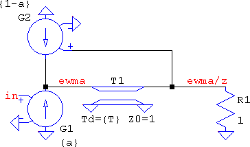
The TLINE version suffers from overshoots and a generally un-clean output, while the shift register is spot on. Imposing a timestep one thousand times lower than the sampling period cures the plague, but only so much. On the other hand, the former can have an "instantaneous" output, whereas the latter needs tinkering with the clock, and .AC is not possible.

For 2nd order transfer functions, in terms of hardware, multipliers are more expensive than delays, but in SPICE the reverse is true. The more delays, the more the timestep is reduced, while multipliers are simple VCCSs. For this matter, the direct form II is the most efficient for IIRs. The element/node count is 6 x VCCS + 2 x TLINE + 2 x R = 10e/5n. This and its behavioural counterpart are compared in 2nd_iir.asc, with a random notch lowpass.

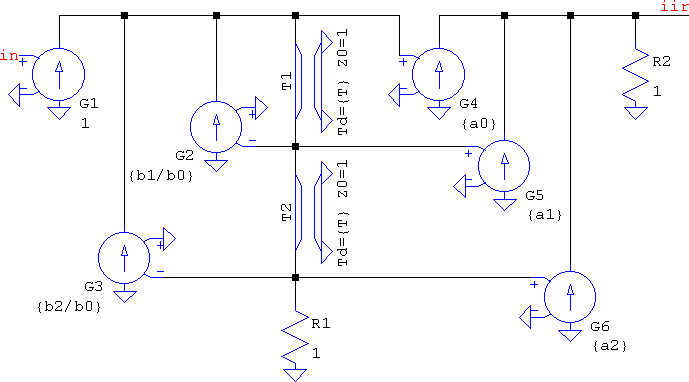
If lowpass to bandpass conversion meant s → (s²+ω₀²)/(s⋅ω_bw) in the analog domain, here it means:

z-1 → −	z-2−[2⋅α⋅k/(k+1)]⋅z-1+(k−1)/(k+1)
	[(k−1)/(k+1)]⋅z-2−[2⋅α⋅k/(k+1)]⋅z-1+1

Ignoring the unknown parameters, that's a full 2nd order IIR and it can't be simplified, which means the tricks that the analog filters used are no longer available. The result is that each delay gets replaced by a biquad. The only simplifications are:

• If coming from the analog side, apply the transform (of whatever kind) to the already converted bandpass or bandstop, resulting in the usual two biquads, or 20e/9n (19e, if the output VCCSs of the first stage are combined with the input VCCS of the second).
• Expand the transfer function such that the resultant is a 4th order stage, implemented by adding 2 more delays and 4 more VCCSs. The element count will be 16e/7n.

So it seems that it's more advantageous to keep the 4th order stage in terms of computation, but a 4th order means 4 delays; the signal may suffer. Which one is better is up to the designer.

---

FIRs

The biggest simplification that can be made in the FIR world is the basic moving average: at its core, it's an equally spaced sampled signal with equal weights, which is nothing but a definite integration. This means a difference of two integrals delayed in time, therefore the response can be approximated with analog elements. An alternative is to first delay the signal and then apply indefinite integration. Mathematically-wise it's the same thing. SPICE-wise, one may be preferred over the other depending on the nature of the signal: if it's noisier, integrate and then delay may tame the erratical behaviour a bit. Or not. It's a matter of choice. There is a third way, to use the recursive formula, which results in two delays and no capacitor (see ma.asc):

H(z)=	1	⋅	1−z-K
	K		1−z-1

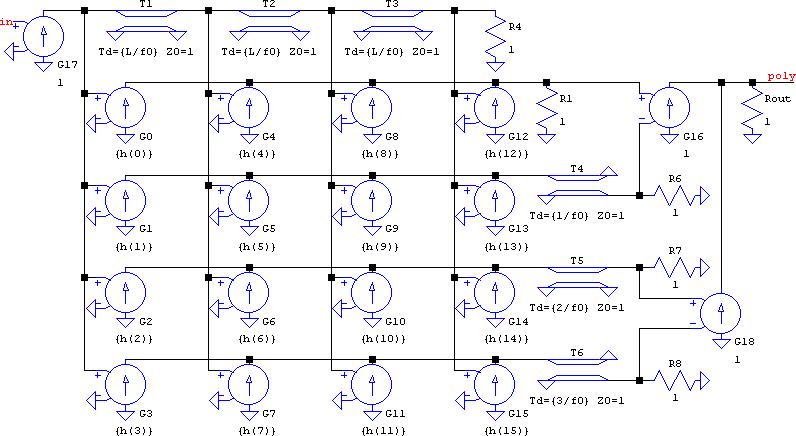
There is some hope for the FIRs, though. Text-book wise, a symmetrical FIR can be used in a folded way, thus halving the number of multipliers. That makes sense in hardware, but since in SPICE it's the delays that slow down more, a different way to simplify is needed: polyphase filtering. The advantage is that the delays not only can be reduced, but their values can also be increased. The disadvantage is that the number of multipliers is the same. However, this comes with a hidden benefit, that of being able to use asymmetrical impulse responses (e.g. minimum phase). In poly.asc there's a 15th order FIR:

---

The need for speed

Efficient, or not, eventually what matters are the results. The signals are supposed to go to, and come from a sampled system, therefore signal conditioning is of concern. This is what sample & holds are for. Even with the signal degradation that comes from the transmission lines, the s&h can help, sometimes a lot. This means there is a need for a clock signal, and this can be inefficient. The usual clock is a PULSE source, and this is (almost) always defined with all its attributes, including rise and fall times. But this is inefficient.

As far as the clock is concerned, the only active part of it is the trigger edge − for the SAMPLEHOLD it's the rising edge − which means specifying anything other than tr and T is useless (td is just a delay). The other values will get their defaults, as defined by LTspice: Ton can be zero and tf will be min(Ton, T−Ton)/10; if Ton is zero, then it's T/10. This results in PULSE 0 1 0 {tr} 0 0 {T}, a clock that's spikey looking, has the same effect as the "usual" one, but is faster because the timestep only has to be reduced around one part, the rising edge; the other timepoints are far apart, relative to the period. And if tf = T - tr, it's a reversed sawtooth that has one less timepoint. If the rising edge has no critical timing then tr can be left null, resulting in two edges, rising and falling, that are 10% of the period, no ON time, and a simulation that's not hindered by the existence of a sharp edge: PULSE 0 1 0 0 0 0 {T}. Though the reversed sawtooth may be a tad faster. And yet, there may be cases where even this can be improved. The SAMPLEHOLD does trigger on the rising edge, but that just means a transition from zero to high, of any kind. If the clock is a SINE source, the timestep will not wait for any sharp transitions other than the s&h's, and those can be relaxed, simulation-wise. But this can be a bit extreme, because in some cases the signal doesn't vary as smooth as we'd like and then the transitions matter: if they are too relaxed, information can be lost. This is particularly true for long simulations, large timespans relative to the period. But even this can be turned into an advantage ...of some sort.

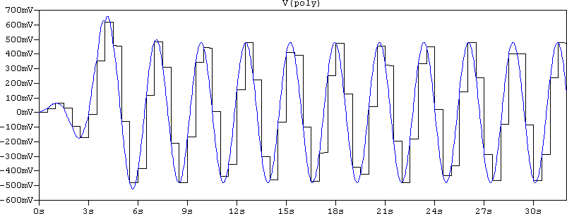
A digital filter implies a sampled signal. But what if the information is the one that's needed, instead of the signal, itself? Think of it this way: before sampling, the signal is analog, then after the filter the signal comes out sampled, but is then filtered. What is approximated here is the output signal before oversampling. But, eventually, that signal will be filtered to recover the analog information. These steps can be skipped. Due to the analog nature of SPICE, despite using transmission lines, a smooth-varying signal at the input will mean a smooth signal at the output. SISO: smooth in, smooth out. If the filters are used for harmonic signals, then the s&h part can be discarded, and the output will be smooth varying (save minor artifacts). Caution: the spectrum folding will be lost, but only in .TRAN; .AC works just fine. For example, in poly.asc, this is how the output looks like when using SINE 0 1 {wc} as the source, with and without sampling:

So far, it has been shown that filters of high to very high orders can be built, and some can even simulate very fast. From here until trying to make a subcircuit with an automated process of calculating some filter is one step. But now there's a new problem. The whole point of this web page was efficiency, even when it was very scarce to find. If the automated process involves a variable order, the schematic that is about to be built must support the maximum number of elements. Which means that if the subcircuit is meant to support a maximum filter order of 10, when run as a 2nd order, only, all the elements up to the 10th order will be useless, at best. The truth is that even if they don't participate to the schematic, even if all the signals are, somehow, deviated to avoid running through the unused elements, they will still be there, encumbering the matrix. And that matrix will consider them as entries, the solver will inevitably leak some numeric residuals in them, in short: they will be used one way or another, slowing down the simulation. The solution is to find a way to disable the unused elements.

This concerns LTspice, in particular. There are two things that LTspice does that can help with this goal:

1. When all the pins of any device (be they primitives or subcircuits) are grounded they are excluded from the matrix, i.e. they are disabled. The exception to these are the current sources, which are meant to deliver no matter what. This can be easily verified by placing any component in the schematic (e.g. a NPN), grounding all the pins, adding .OP, and then click on "run". LTspice will pop an error dialog saying: This circuit does not contain a node other than node "0" (GND). If Generate Expanded Netlist is checked in the Control Panel > Operation tab, or there is an .opt list in the schematic, the netlist entry for the transistor will appear as:

   *1 0 0 0 0 npn

   The * in the beginning means that line is commented out, thus it's not part of the netlist.
2. Node names can be evaluated. They are used as regular character labels, but they can evaluate to a number. 00 and 0 are two different node names, but they both evaluate (the curly braces) to zero. For example:

   V1 00 0 1
   B1 x 0 V=V(00)
   B2 y 0 V=V({00})

   The output of .OP is this:

   V(00): 1 voltage
   V(x): 1 voltage
   V(y): 0 voltage

Even if the GUI doesn't allow it, these two can be combined. No matter what it is, netlist or schematic (.asc), editing is possible and nodes can be assigned parameters, or functions, but not time-dependent; parameter evaluation must be done before the actual simulation. But(!), they must be enclosed in curly braces, otherwise they will be considered generic labels. A very good example is (regretably late) analogspiceman's↗ 3-to-1.asc. For .asc files though, there is a downside: once edited, hovering the mouse over the node will show the name of the node as if the curly braces were part of it; it will not show the evaluated node. So all this is best used in netlists, or for subcircuits.